Electrical Resistivity Tomography (ERT)

ERT · Resistivity method · Electrical survey

Electrical Resistivity Tomography (ERT)

From edge acquisition, direct GD-device connection and proprietary online inversion, to scatter-point QC, mesh blanking, moisture-content and phreatic-line interpretation, and 3D deliverables — the complete ERT loop, with no third-party inversion software.

Supported arrays: Wenner / Schlumberger / dipole-dipole

Request a trial

Overall workspace of the DIGspace electrical method module

Six core modules covering the full resistivity-method lifecycle

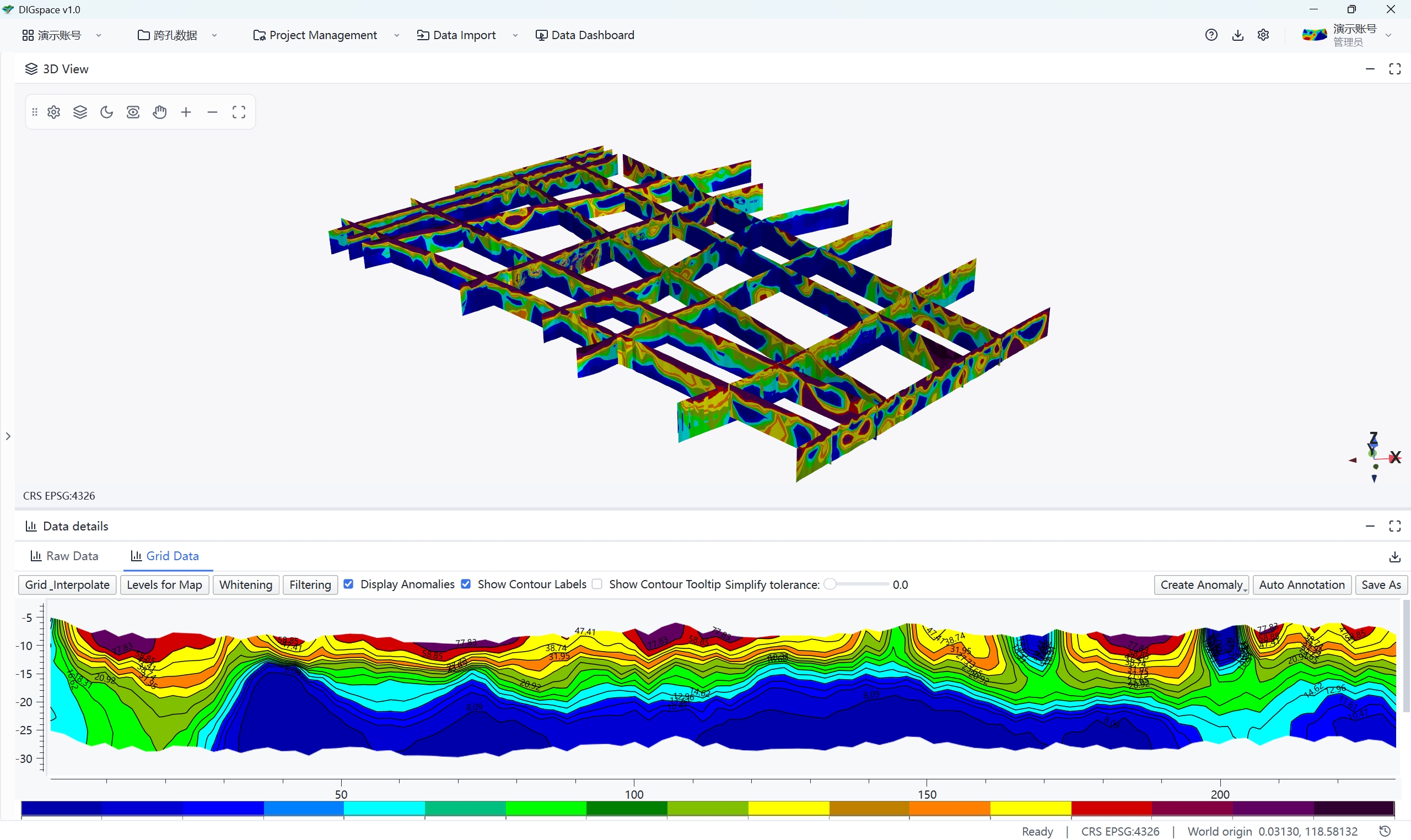
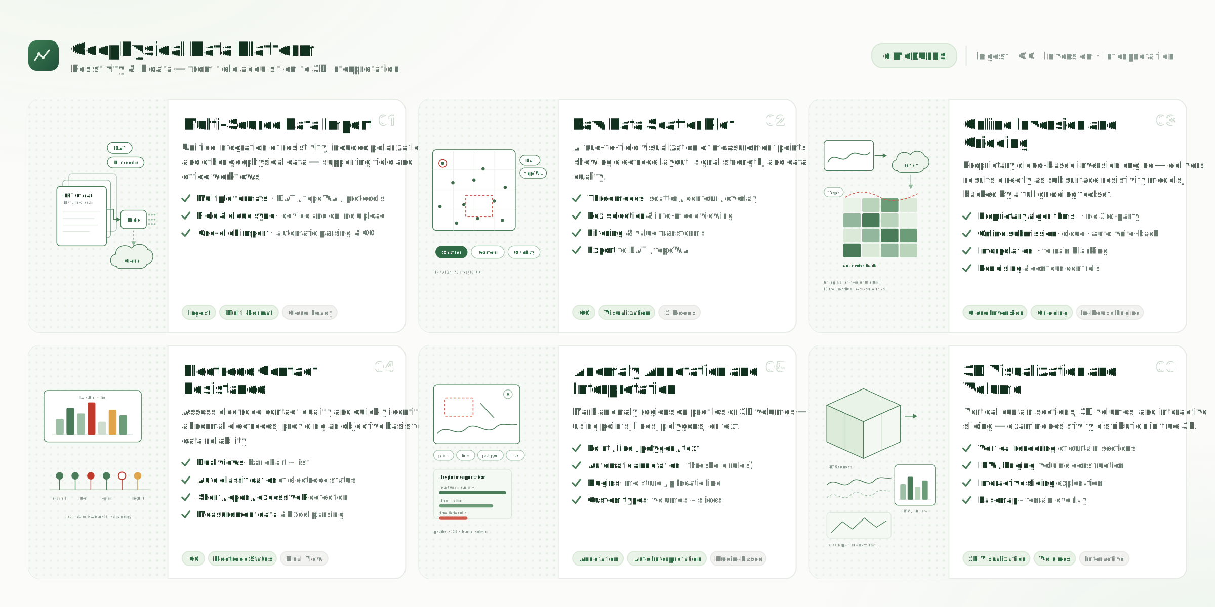
From data import to 3D results export, every step has its professional tool — the content below is organized in three layers: Basics, Core, and Highlights.

Four levels that organize every survey line clearly

Project → Survey Area → Survey Line → Dataset — an object tree that mirrors real project structure

🏢
Project
🗺️
Survey Area / Task
📏
Survey Line
📦
Electrical Dataset

Flexible intake for multiple data sources

Supports online EDGE acquisition, raw device data, inversion result files, and common standard formats; electrode spacing and array type are parsed automatically on import.

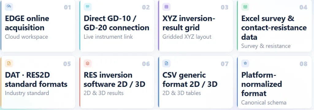
Four import methods covering every data source

From automatic online EDGE acquisition to SD cards and inversion result files — flexible intake with a clear, controllable flow.

Online EDGE acquisition
Online EDGE acquisition
Once the field EDGE unit connects to the instrument, measurement data is acquired automatically and uploaded to the platform on schedule over the network — no manual card retrieval or copying. Resumable transfer is supported, and data enters QC and inversion as soon as it arrives.
📂 Device Data Import
Scan an SD card or a local folder, filter by result type (resistivity / apparent resistivity / sounding / borehole), with support for merging multiple survey lines and repairing corrupted files.
📄 Inversion Result Import
Supports xyz files and inversion result Excel sheets, parsing three tables — measurement data, contact resistance, and survey line header information — with automatic parameter recognition and format conversion.
📌 Trajectory Import
Each survey line imports its own trajectory file (.xlsx); assign a coordinate system and it links automatically to the matching dataset. If a trajectory already exists, you are prompted before overwriting.

Raw data scatter plot — measurement quality at a glance

A true-to-field visualization of acquired points, helping you review electrode layout, signal strength, and contact quality.

Info Mode

Click a scatter point to view electrode number, signal, resistance, pseudo-resistance, and other details, and quickly locate abnormal measurement points.

Box-Select Browse

Drag a box to select a group of measurement points and inspect their distribution and values together, flexibly focusing on any area of interest.

Electrode Selection

Click an electrode along the top of the profile to automatically look up its related measurement points — the electrode-to-data relationship is clear at a glance.

Three Display Modes

Switch freely among scatter, Kriging contour, and overlay views. Value transforms support linear, inverse, logarithmic, and other mathematical transforms.

Equal-Aspect Display

Identical horizontal and vertical scaling prevents geometric distortion; the color band renders independently in the background and stays sharp at every zoom level.

Data Export

Processed measurement data can be exported to DAT / topoWA for direct use in downstream steps.

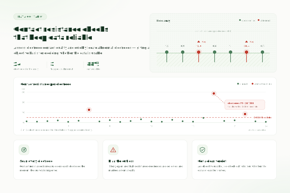
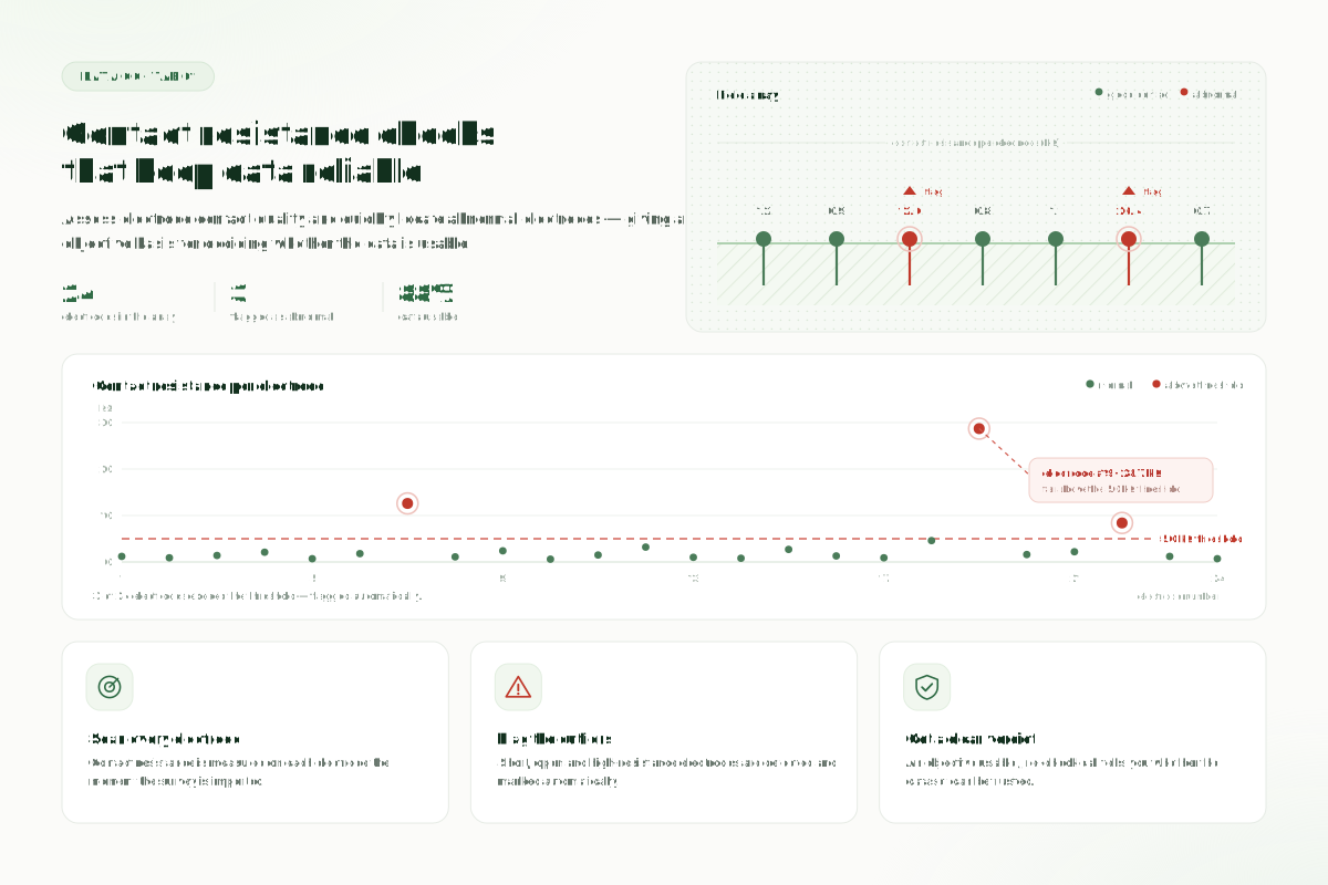
Contact-resistance check · verify data reliability before inversion

Assess electrode contact quality and quickly locate abnormal electrodes with shorts, open circuits or excessive resistance

Gridded contour map — the core view of resistivity distribution

Gridding, blanking, and filtering of inversion results — from a resistivity model to a deliverable profile.

Gridded contour map — the core view of resistivity distribution

Resistivity-method gridded isosurface profile

Illustration · ERT inverted resistivity profile with low-resistivity anomaly annotation (values shown are illustrative).

Gridding

Interpolate scatter points into a regular resistivity grid, with multiple interpolation methods and adjustable grid density and boundary determination.

Terrain Blanking

Mark specific regions as invalid data and remove them: automatic boundary detection / blanking file import / model masking, with trapezoidal or rectangular clipping.

Filtering

Smoothing, sharpening, denoising, and other filter operations, with adjustable filter type matrix, edge handling, null-value handling, and number of passes. Settings can be saved and reused.

Core

A results production system built around the proprietary cloud-based inversion engine — proprietary algorithms, from inversion to 3D results without relying on third-party software.

Proprietary cloud-based inversion engine — an end-to-end closed loop unique in the industry

Inversion is the core step in resistivity method work. With proprietary algorithms running online, DIGspace no longer needs any third-party inversion software.

Proprietary Algorithms

The core inversion algorithms are fully proprietary, optimized for the ERT acquisition system and the data characteristics of GD devices, with no reliance on third-party inversion software.

Online Computing

Submit inversion jobs in the browser with template-based parameter configuration and online progress tracking — no local high-performance workstation required. Launch directly from the scatter plot.

Closed-Loop Results

Inversion results are automatically written back to the dataset and flow directly into gridding, 3D volumes, and plugin analysis — no file export-and-import, and the process is fully traceable.

Monitoring Support

Each acquisition round automatically triggers inversion and ingests the results, serving long-term online monitoring of dams, embankments and slopes; threshold rules judge anomalies automatically and generate alerts.

Inverted fence sections from multiple ERT survey lines stand upright in 3D space

Actual product UI · multi-line fence sections together with surface imagery

Anomaly annotation and management — the full workflow from discovery to location

Mark areas of interest on profiles or 3D volumes, with multiple shapes and automatic detection.

Multiple Annotation Shapes

Four annotation methods — point, line, polygon, and text — drawn directly on the figure, with support for manual coordinate entry and subsequent editing.

Automatic Annotation

Configure threshold rules (absolute value or percentage) and minimum point count, run automatic detection with one click, and save after confirming the results list.

Anomaly List Management

Centrally manage every annotation on the current figure: show / hide, delete, view details, and locate an anomaly with one click.

1
Create anomaly
Choose a shape type, draw on the figure or enter coordinates, and fill in name, notes, and properties.
2
Property editing
Fill in anomaly type, physical properties (length / width / burial depth), and coordinate system information, and add screenshot previews.
3
List management
Anomalies are managed centrally in a list, with show / hide, delete, details, and jump-to-anomaly-location.
4
3D annotation
Create anomalies on 3D curtain sections, slices, and depth bands, with automatic selection of 2D / 3D rendering.

Cavity

Water-Bearing Zone

Loose Zone

Utilities

Layer / Horizon

Profile anomaly markup and properties panel

Delineating anomalies on a profile with the properties panel · anomaly type, physical properties (length / width / burial depth), and screenshots are archived together with the anomaly.

From curtain sections to volumes — a three-dimensional presentation of resistivity distribution

2D profiles answer what is in this section; 3D views answer how it is distributed in space.

Most used: inversion fence sections

Each survey line's inversion result stands vertically at its true position, arranged like a row of curtains. ⭐ Most Commonly Used

Inversion curtain sections

Advanced analysis: 3D volume rendering

IDW / Kriging interpolation builds a 3D resistivity volume, displayed semi-transparently to reveal internal structure. Advanced analysis

3D volume rendering

Result display: anomaly-volume overlay

Interpreted anomalies are displayed as 3D markers, showing their spatial distribution and interrelationships. Results presentation

Anomalous body overlay

Spatial positioning: basemap + terrain

Imagery and digital elevation model basemaps, with image texture and elevation relief draped over 3D terrain. Spatial positioning

Base map and 3D terrain

QC aid: plan-view footprint

Horizontal survey line traces plus electrode marker points, laid flat on the ground to show survey line layout. QC aid

Survey-line plan-view footprints

Highlights

Differentiating capabilities that others lack — or cannot deliver with the same experience.

View Analysis Workbench · Six Distinctive Highlights

The core workbench on the ERT dataset detail page: invert only clean data, watch the inversion process, and rely on traceable results — six capabilities linked into a data-trust pipeline.

🧹
Data preprocessing
Keep dirty data out before inversion
📊
Two views in one
See the raw distribution clearly
🎨
Smart color scales
A unified color language
🔲
One-click mesh
Set the stage for inversion
⚡
Iterative inversion
A transparent, trustworthy process
✅
Linked error analysis
Results that stand up to review

Data preprocessing: keep "dirty data" out before inversion

The reliability of inversion results depends three parts on the algorithm and seven parts on the data. The workbench includes a complete "clean first, then invert" toolchain.

Data preprocessing: keep "dirty data" out before inversion

Capability	How to use	What it solves
Data filtering	Batch-filter measurement points by value range or conditional expressions.	Remove obvious out-of-range, negative, and NaN "wild points" with one click.
Data cleaning	Multi-mode anomaly detection: IQR quartile / standard deviation / MAD / custom threshold.	Robustly identify outliers without relying on personal rule-of-thumb values.
Manual point deletion (hide)	Click or box-select measurement points → Hide, with the hiding persisted.	Apply field experience to flexibly handle individual points that "just look wrong."
Fast ABMN electrode point filtering	Click an electrode atop the profile → automatically look up all related A / B / M / N measurement points → hide with one click.	When an electrode has poor contact, hide its dozens of related points as a group instead of picking them one by one.
Zoom-box point deletion	Scroll to zoom → box-select → Hide.	Pinpoint accurately even in dense scatter areas and avoid accidental deletion.

Two charts in one: scatter + contour with live interpolation preview

Three Display Modes

Scatter plot (color-mapped raw measurement points), contour plot (Kriging-interpolated resistivity contours), and overlay plot (point positions, values, and their contours compared on one screen).

Live Interpolation Preview

Switching display modes instantly recomputes and renders, with no job submission and no waiting; the judgment of "whether to interpolate and which method to use" is completed on the same screen.

Layered Drawing · High-Definition Color Band

Electrode diamond markers and data blocks are drawn on separate layers to avoid occlusion; the color band is cached and rendered independently in the background, staying sharp no matter how you zoom.

No need to switch back and forth between the "scatter plot" and the "contour plot" — both forms appear on the same screen, and parameter adjustments are seen immediately.

Gallery

Scatter + contour overlay map

Scatter + contour overlay · two charts in one, with Kriging contours and raw points compared on the same screen and instant recomputation on switch.

Smart color scale: histogram distribution + one-click preset application

Color is more than decoration — it is a data language. The color scale editor turns the "color scheme" from a black box into a quantifiable, reusable engineering asset.

Three Distribution Modes

LinearEqual-interval classes, suited to evenly distributed data;Loglogarithmic classes, suited to resistivity data spanning multiple orders of magnitude;Equal-areaevenly split by frequency, with each color class corresponding to the same number of measurement points.

Live Histogram Linkage

The top histogram shows the true data distribution; dragging color-scale nodes highlights the current data range in sync. Opacity supports custom / gradient / Level Ends, and stretching can be set to none / bidirectional / custom.

One-Click Preset Management

The current color scheme can be "saved as a preset"; historical presets switch in one click and can be imported / exported for team sharing — multiple institutes and projects get one common color language for their sections.

Smart color-scale editor

Smart color scale editor · live histogram linkage, Linear / Log / Equal-area modes + preset management

One-click mesh generation: quickly build an inversion model from preprocessed data

From "scatter plot" to "inversion stage" is just one click away.

Direct Entry

The "Data Inversion" toolbar button expands the inversion operation area with one click — no page switching and no separate software.

Four Core Parameters

Model depth, maximum cell area, number of nodes between electrodes, and horizontal extension range; defaults are computed automatically from the data, so even new users can start directly.

Live Preview · Persistent State

The 3D view displays the mesh, electrode positions, and axes in sync, and the status bar reports ready / generating / success / failed in real time; repeatedly opening and closing the panel never loses the mesh.

One-click inversion mesh generation

One-click mesh generation · 4 adjustable parameters + live 3D preview + electrode positions on screen — engineers no longer run inversions blind.

Automatic iterative inversion: transparent process, dynamically visible error

Inversion is no longer a "black box" — every iteration's result, error, and convergence trend are all laid out in front of the user.

Ten Parameters for Flexible Adjustment

Regularization factor Lambda, maximum number of iterations, initial model resistivity, robust weighting, blocky model constraint, zWeight, minimum / maximum resistivity (with validity checks), water body parameters, and more.

Real-Time Iteration-by-Iteration Display

The toolbar displays "Iteration: 6 / Misfit rRMS: 29.04%" in real time, and the preview refreshes with each iteration under a unified color-scale range to ensure comparability; it follows the latest frame by default, and manually selecting a frame stops following.

Iteration Playback + Whiteout Angle

Use the dropdown to review any N-th iteration result and compare the convergence process; manual adjustment of color-scale upper and lower limits changes display only, not computation; the Whiteout angle removes unreliable shallow zones.

Automatic iterative inversion

Automatic iterative inversion · number of iterations and rRMS error shown in real time — shifting from "click start and wait" to "watch it converge and step in anytime."

Error analysis + interactive point rejection: results that stand up to review

Inversion is not the end point; being able to explain the inversion is. "Which points fit poorly" changes from hidden information into a visible, actionable object.

Error Analysis Panel

The upper relative-error pseudosection aligns with the original scatter points by A / B / M / N, with darker colors indicating poorer fits; below are a relative-error histogram and a draggable threshold line; the top shows statistics for valid measurement point count, average error, RMS, and maximum error.

Linked Highlighting

Drag the threshold line, and above-threshold points in the scatter plot gray out in real time with a synced count; grayed points are candidates for rejection, with no back-and-forth comparison between two windows.

Quick Rejection · Re-Invert

Without leaving the current operation: select grayed points → Hide → rerun the inversion, and error statistics refresh immediately. The "clean — invert — verify — clean again — re-invert" loop continues until the error is acceptable.

Error analysis and linked rejection

Error analysis + interactive point rejection · error pseudosection + histogram threshold line + linked graying of scatter points — invert until the "error is acceptable."

Experience comparison with traditional desktop ERT software

Dimension	Traditional desktop ERT software	DIGspace view analysis workbench
Data cleaning	Mostly manual processing in Excel / scripts	Built into the toolbar: filtering / cleaning / hiding / box selection / electrode lookup in one
Scatter ↔ contour	Switching between two windows	Two charts in one screen, overlay-mode comparison, instant recompute on switch
Color scale management	Built into the software; not customizable or reusable	Live histogram linkage + preset saving, one-click application, team sharing
Mesh generation	Hidden parameters; manual trial calculation needed	4 adjustable parameters + live 3D preview + clear status feedback
Inversion process	A black box; results known only after the run finishes	Dual entry with proprietary online engine + local fine-tuning; every iteration is visible and reviewable
Error analysis	Usually a standalone tool with no linkage	Threshold line linked to the scatter plot; reject with one click and go straight into the next inversion round

Device ecosystem · unattended operation · direct engineering conclusions

Beyond the view analysis workbench, DIGspace ERT offers three additional platform-level differentiators.

Edge online acquisition: unattended; inversion starts when data arrives

Once the instrument is connected at the edge, survey data is acquired automatically on schedule and uploaded to the platform over the network — no manual card retrieval or copying; if the network drops, transfer resumes automatically, and on arrival the data enters exactly the same preview, QC and inversion flow as a manual import. Together with the proprietary cloud inversion engine this fully automates the monitoring loop of "acquisition — upload — inversion — anomaly detection — alerting", and is particularly suited to long-term unattended scenarios such as reservoir dams, dams and slopes.

Direct GD-device connection: from field to cloud in three steps

Geomative GD series devices are deeply integrated with DIGspace: scan the device QR code for automatic recognition, measurement data is converted to standard format automatically, and data submission is completed in three steps. Built-in quality checks run during upload — bad-point detection, duplicate data recognition, automatic array type matching, and contact resistance status classification — so data is usable the moment it enters the library, eliminating much of the manual format conversion and data cleaning work in traditional workflows.

External-plugin business analysis: from resistivity results straight to engineering conclusions

The inverted resistivity model is not the end point. Business-analysis algorithms such as automatic moisture-content calculation and automatic phreatic-line (saturation-line) identification run as external plugins on top of the platform data: using geotechnical property parameters they convert moisture-content sections automatically, delineate the boundary between saturated and unsaturated zones and output the phreatic-line position, with manual review and adjustment supported — directly feeding seepage-stability assessment and anomaly alerts. Plugin results are managed together with resistivity sections and 3D volumes inside one project and can flow directly into reports and online-monitoring dashboards; the platform can also keep mounting more partners' dedicated analysis plugins.

Complete the full ERT workflow in four steps

From data intake to results delivery, every step is completed within the DIGspace platform — no software switching.

1
Data intake
Automatic EDGE acquisition / direct GD connection / common-format import, with dual QC via scatter plot + contact resistance.
2
Inversion mapping
Dual entry — proprietary cloud online inversion (batch / online submission) and local fine-tuning; gridding → blanking filter → section generation
3
Anomaly interpretation
2D sections + 3D volumes + slice analysis; delineate anomalies, classify and archive; plugins interpret moisture content / phreatic line automatically
4
Results delivery
Multi-format results output: images / data / vector / 3D volumes / reports.

ERT + GPR + boreholes — the platform value multiplier

⚡ ERT electrical + 📡 GPR radar = deep and shallow complement each other, properties cross-confirm; a single method is ambiguous — multi-method combination is DIGspace's core advantage.

Electrical Resistivity Tomography (ERT) · typical applications

Great depth, sensitive to moisture content, capable of long-term online monitoring — ERT is irreplaceable in these scenarios. Below are the pain points, method configurations, deliverables and cases for typical scenarios.

Reservoir dam & embankment operation inspection and monitoring

Periodic survey + long-term online monitoring · automatic inversion and threshold alerts; moisture content / phreatic line interpreted automatically ERT Seepage field Online monitoring Monitoring · Long-term

Slope Monitoring

Time-varying resistivity captures landslide precursors · moisture change and slip-zone identification. ERT GNSS displacement Tiered early warning Monitoring · Long-term

Landfill Leakage Monitoring

Precise liner leakage location: environmental risks found and handled early ERT Leak localization Environmental compliance Monitoring · Long-term

Engineering Investigation

Karst, cavity, and mined-out zone detection · multi-method joint investigation improves both efficiency and accuracy. ERT GPR Borehole data Investigation · Project-based

Hydrogeology

Resistivity inversion plus parameter conversion characterizes aquifers and groundwater flow fields. ERT Property conversion 3D modeling Investigation · Project-based

Tunnel Look-Ahead Prediction

Multi-method integration to identify adverse geology and water-bearing structures ahead of the tunnel face ERT GPR Joint interpretation Investigation · Along the construction schedule

Frequently asked questions about ERT

Poor electrode grounding is the number-one killer of electrical survey data quality. The platform provides bar-chart and list tabs: in the bar chart, each electrode is one bar whose height is its resistance, so bad electrodes stand out at a glance; the list gives complete details of electrode number, timestamp, resistance and EMF, with filtering by status. The system automatically classifies electrodes into three states — normal, short/open circuit, and excessive resistance — so crews can decide on site which electrode needs watering or re-driving, instead of discovering unusable data back in the office.

The desktop local inversion workbench runs on an ordinary office computer; a routine section inversion completes within minutes. The proprietary cloud online-inversion engine does not depend on local hardware: submit a job in the browser and it computes in the background, with iteration progress and rRMS error viewable at any time. Cloud compute is recommended for batch inversion and for automatic inversion tasks in long-term monitoring.

There are three core differences. First, the inversion engine is developed in-house by DIGspace and runs online in the cloud, independent of third-party inversion software; batch inversion and automatic monitoring inversion complete unattended in the background. Second, the process is transparent — iteration count, rRMS error and convergence trend are visible iteration by iteration, and any round can be revisited. Third, results form a closed loop: inversion outputs are written back to the data set automatically and flow straight into gridding, 3D volumes and the moisture-content / phreatic-line plugin analyses, with no export-and-reimport. The desktop also provides a local inversion workbench for iteration-by-iteration fine-tuning, sharing the same data store as the cloud engine and complementing it.

Yes. Business-analysis capabilities are delivered as external plugins: the moisture-content plugin uses geotechnical property parameters to convert and generate moisture-content sections and spatial distributions; the phreatic-line plugin automatically delineates the saturated / unsaturated boundary and outputs the phreatic-line (saturation-line) position, with manual review and adjustment supported. Plugin results are managed together with resistivity sections and 3D volumes inside one project and can flow directly into reports and online-monitoring dashboards; the platform also supports continuously mounting more business-analysis plugins.

Masking is not simply cutting away the picture; it marks the area above terrain as "invalid data" and excludes it from subsequent computation and rendering. The platform offers three methods: automatic boundary-based determination, mask file import, and model-based masking, with trapezoidal or rectangular cropping supported. Masked profiles drape naturally onto the real ground surface in 3D scenes, with no misleading "profiles hanging in mid-air" or "data growing above the ground."

3D volumes are generated from multiple 2D profiles using IDW (inverse distance weighting) or Kriging interpolation; accuracy depends on profile spacing and data density — the denser the profiles, the higher the volume accuracy. Convex-hull boundary handling prevents over-interpretation of extrapolated areas. Volumes are recommended for overall spatial-distribution trend analysis and anomaly localization; detailed interpretation should still rely on the original profiles.

Fully supported. ERT is one of DIGspace's primary methods for online monitoring: edge online devices acquire automatically with resumable transfer and synchronized ingestion; together with the proprietary cloud inversion engine, anomalies are detected automatically and alerts pushed — the whole flow from acquisition to alert push is automated, and plugins can output moisture-content sections and phreatic-line positions automatically. Long-term monitoring scenarios are already in service, including reservoir-dam O&M, dam seepage, slopes and municipal landfills.

Frequently asked questions about ERT

Want to experience DIGspace ERT yourself?

Book an online demo — we will walk through the complete workflow on your scenario

Request a 30-day trial